Time series analysis is a specialized branch of statistics that deals with the examination of ordered, often temporal data. It has a wide range of applications across various disciplines, such as economics, finance, and weather forecasting, among others. This type of analysis involves studying data points that are collected in a chronological order, allowing researchers to uncover patterns, trends, and anomalies in the data and make predictions based on historical information.

In time series analysis, data points are usually collected at regular intervals, which allows for the study of time-dependent relationships between variables. This helps researchers reveal any underlying structure or cyclic behavior that might exist in the data, and also enables them to identify seasonal fluctuations and trends. Additionally, time series can help analysts forecast future values of a variable based on historical information, which is especially important in fields like finance, where accurate predictions can lead to significant gains or losses.

There are various techniques and methods used in time series analysis to examine patterns and irregularities present in the data. Depending on the context, analysts may choose to explore different types of analysis, such as exploratory analysis, which helps describe and explain observations in a given time period, or more advanced modeling approaches like the naive forecast method. This method involves using the value from the previous period as a reference, providing a straightforward, yet informative means of analysis. Overall, time series analysis serves as a valuable tool for various industries and fields, helping make sense of ever-changing data and assisting decision-makers in drawing informed conclusions.

A brief explanation of the concept of Time Series Analysis:

Time series analysis is a powerful and crucial statistical method used in data analysis, particularly when dealing with sequential data. It involves analyzing data points, such as observations or measurements, that are collected at regular time intervals. From financial stock prices, sales data, and weather forecasts to web traffic analytics, time series data is ubiquitous in real-world applications.

Imagine tracking the number of visitors on a website. Each day, you record the number of users who visit your site, creating a series of data points over time. This is a classic example of a time series. Analyzing this data isn’t just about understanding how many users visited your site in the past; it’s about using this past data to predict future web traffic trends, inform business strategies, optimize resources, and ultimately drive business growth.

Understanding time series analysis is crucial for data analysts because it opens up a world of insights from temporal data that otherwise would be difficult to glean from static datasets. By unearthing patterns and trends, time series analysis can help forecast future events, allowing businesses to make informed, proactive decisions.

In the following sections, we will delve into the details of time series analysis, its importance, key concepts, various methods, and its application in data science and machine learning. Whether you’re a beginner or looking to enhance your knowledge, this comprehensive guide aims to provide a solid foundation in understanding and implementing time series analysis.

Importance and Significance of Time Series Analysis for Data Analysts

In the vast world of data analytics, time series analysis holds a position of paramount importance. The significance of this statistical technique lies in its ability to uncover hidden patterns within sequential data, enabling data analysts to forecast future trends based on historical data.

Time series analysis allows for an in-depth exploration of data.

Data analysts can extract meaningful insights about systematic trends, seasonal variations, and unexpected shifts, which may otherwise be challenging to spot. Understanding these patterns can significantly enhance the clarity of complex data and help make sense of the noise.

Time series analysis is a powerful tool for forecasting.

By identifying data patterns that repeat over time, analysts can predict future data points with a certain degree of confidence. In the business world, this can be incredibly beneficial for various functions such as sales forecasting, inventory management, financial planning, and operational strategies. For instance, by predicting web traffic trends, businesses can optimize their marketing strategies, allocate resources more effectively, and improve user experience.

Time series analysis helps in decision making and strategy formation.

Providing an evidence-based outlook on the future supports decision-makers to plan strategically. It removes a significant element of uncertainty and risk from the decision-making process, enabling organizations to be proactive rather than reactive.

Time series analysis serves as a cornerstone for many predictive models.

It’s an indispensable tool for analysts working with machine learning algorithms, especially in areas like algorithmic trading, predictive maintenance, weather forecasting, and even in the medical field for predicting disease spread.

Understanding Time Series

As we delve deeper into the realm of time series analysis, it’s crucial to grasp the foundational concepts that underpin this field. In this section, we’ll explore what exactly a time series is, familiarize ourselves with essential time series terminology, and examine real-world examples of time series data. We’ll also delve into the different data types you may encounter in time series analysis. By understanding these fundamental concepts, you’ll be well-equipped to explore the more advanced facets of time series analysis. Whether you’re a novice analyst or an experienced professional seeking a refresher, this section aims to solidify your understanding of these basic, yet crucial, concepts.

Definition of a Time Series

In its simplest form, a time series is a sequence of data points collected at consistent time intervals. These intervals could be seconds, minutes, hours, days, weeks, months, or even years. Each data point in the series corresponds to a specific moment in time.

Think of it like a timeline where you jot down particular measurements as they happen. For instance, if you record the temperature every hour, or monitor daily stock prices, or count the number of website visitors each day, all these are examples of time series.

The defining feature of time series data is its order. Unlike other data types, the sequence of data points in a time series matters significantly as it reflects the temporal order of events. This is what makes time series data unique and why we require special techniques, like time series analysis, to study it.

By breaking down time series into this simple definition, it’s easier to see why it’s such a common type of data and why understanding it is so crucial for data analysts. It’s a type of data we encounter regularly in various fields, from business and economics to science and technology.

Time Series Terminology

Understanding the language of time series analysis is essential for gaining proficiency in this field. Here are some commonly used terms that you’ll encounter in your time series journey:

1. Trend: A trend represents a long-term increase or decrease in the data. It’s the overall direction that your data is taking over time. For example, a steadily growing website’s monthly user count shows an upward trend.
2. Seasonality: This refers to predictable and recurring patterns or cycles in time series data that happen within one year. For example, retail sales often increase in November and December due to the holiday season – this is seasonality.
3. Cycles: Cycles are fluctuations in the data that are not of a fixed period. They happen when the data rise and fall irregularly, irrespective of the season. For instance, economic cycles of boom and recession.
4. Stationarity: A time series is said to be stationary if its statistical properties do not change over time. In other words, it has constant mean and variance, and its covariance is independent of time. Most time series models assume that the data is stationary.
5. Autocorrelation: This is a statistical correlation that measures the relationship between a variable’s current value and its past values. For example, if a website’s traffic today is high, autocorrelation would measure the likelihood that the traffic will be high tomorrow too.
6. Lag: Lag is a fixed period of passing time between two related occurrences in time series data. In other words, it’s a term used to describe a specific time shift in the data. For example, we might use a lag of 7 to compare traffic data from one week to the previous week.
7. White Noise: This term refers to a series of random variables where each variable has a mean of zero, constant variance, and zero correlation with all other variables in the series.

Data Types in Time Series

In the context of time series analysis, data can be broadly classified into two types:

1. Univariate Time Series: A univariate time series consists of single observations recorded sequentially over equal time increments. In simple terms, you’re observing one variable over time. For instance, tracking the daily temperature in a city or monitoring the daily closing prices of a stock creates a univariate time series. It’s univariate because we’re only observing one variable – either temperature or stock prices.
2. Multivariate Time Series: A multivariate time series, as the name suggests, consists of multiple variables recorded at the same time intervals. Here, instead of just one set of observations, we have multiple, and the relationship between these variables becomes important. For example, if you’re tracking both the daily temperature and the amount of ice cream sold at a local store, that would create a multivariate time series. It’s multivariate because there are multiple variables at play, and understanding the relationship between these variables (like how temperature affects ice cream sales) is a significant part of the analysis.

Knowing whether your time series data is univariate or multivariate is important because it affects the kind of models and analytical approaches you would use. While univariate time series analysis is simpler and more straightforward, multivariate time series analysis allows for a richer understanding of complex systems where variables interact with each other.

How to Analyze Time Series?

Embarking on the journey of analyzing a time series may seem daunting at first, but having a structured process in place can make it much easier. In this section, we’ll break down the process flow of time series analysis and familiarize ourselves with its key components: trend, seasonality, cycles, and the irregular component. Understanding these core elements of time series analysis will equip you with the necessary knowledge to delve deeper into the subject and apply your skills to real-world data.

Let’s begin by exploring the step-by-step process of conducting a time series analysis.

Process Flow of Time Series Analysis

1. Data Collection

The first step is gathering your time series data. This could come from various sources like logs, sensors, databases, or APIs. Ensure the data is collected at consistent time intervals and is organized in chronological order.

2. Data Cleaning and Preprocessing

This step involves making sure your data is clean and ready for analysis. This could mean dealing with missing values, outliers, or any irregularities in the data. The goal is to make sure your time series is accurate and reliable for further analysis.

3. Visualization

Visualizing your data can give you a lot of insight into your time series. Plots can help identify trends, seasonality, outliers, and more. It’s a quick and easy way to understand the overall pattern and structure of your data.

4. Testing for Stationarity

Many time series models assume that the data is stationary, meaning the mean and variance are constant over time. Therefore, it’s important to test your data for stationarity. If the data is not stationary, transformations may be needed.

5. Model Selection

There are many models for time series analysis and forecasting, such as ARIMA, SARIMA, Holt-Winters, etc. The choice depends on your data and the specific application. The selected model should be able to capture the patterns in your data effectively.

6. Model Fitting

Once the model is selected, the next step is to fit the model to your data. This involves using your data to estimate the parameters of your chosen model.

7. Model Evaluation

After fitting your model, you need to assess how well it works. This usually involves comparing the predicted values to the actual values and using error metrics such as Mean Absolute Error (MAE), Mean Squared Error (MSE), or Root Mean Squared Error (RMSE).

8. Forecasting

Once you are satisfied with your model, you can use it to forecast future values. Depending on your model, you can even provide a confidence interval for your forecasts.

9. Model Updating

Time series analysis is not a one-time process. As new data becomes available, the model needs to be updated and re-evaluated. This helps to ensure that the model stays accurate and relevant.

While the specific steps might vary slightly depending on the specific context and data at hand, this general process provides a solid framework for carrying out time series analysis. Each step is essential in its own right and contributes to the successful application of time series analysis.

Components of Time Series Analysis: Trend, Seasonality, Cycles, Irregular Component

A time series can be thought of as a combination of four components. Understanding these components is crucial in time series analysis, as it forms the basis for decomposing and understanding the patterns in our data:

1. Trend: The trend component represents the overall direction that the time series is taking over the long term. It’s the general increase or decrease that we see over time. For example, if there’s a general increase in the number of users visiting a website over several months or years, we would say there’s an upward trend in the data.
2. Seasonality: Seasonality refers to regular and predictable changes in a time series that occur within a specific period (usually within a year). For instance, higher retail sales every December, lower web traffic on weekends, or increased energy consumption in the summer months are all examples of seasonality.
3. Cycles: Unlike seasonality, cycles are fluctuations in the data that do not have a fixed period. They represent repeated but non-periodic oscillations. For example, economic cycles, which include periods of economic expansion and recession, are often seen in financial time series data.
4. Irregular Component (or Residual): After the trend, seasonality, and cyclical components have been accounted for, the remaining part of the time series is known as the irregular, or noise, or residual component. This component is unpredictable, random, and contains no pattern.

In time series analysis, we often decompose the series into these components to understand the underlying patterns better. Each of these components provides us with different insights, and together, they give us a comprehensive picture of our time series data. As a data analyst, being able to identify and interpret these components can be crucial in making forecasts or identifying anomalies in your data.

Significance of Time Series Analysis

Understanding why time series analysis matters and what benefits it brings to the table can add context and value to our practical application of this technique. In this section, we’ll explore the advantages of conducting time series analysis, the reasons why organizations across various sectors use it as a valuable tool, and the limitations we should be aware of when working with time series data. This balanced perspective will allow you to better appreciate the real-world implications of time series analysis and its place in the data analyst’s toolkit.

Benefits of Time Series Analysis

Time series analysis comes with a plethora of advantages for data analysts. It’s not just a statistical technique; it’s a practical tool that can uncover invaluable insights from a variety of data. Here are some key benefits:

1. Forecasting: Perhaps the most significant benefit of time series analysis is its ability to forecast future values based on historical data. This is incredibly useful in numerous fields, from predicting stock prices in finance to forecasting product demand in retail.
2. Understanding Trends and Patterns: Time series analysis helps us identify underlying trends and patterns in data, such as growth trends or seasonal fluctuations. This understanding can guide decision-making and strategic planning.
3. Anomaly Detection: Time series analysis can help identify anomalies or outliers in your data. For example, if your website traffic suddenly spikes, time series analysis can help spot this anomaly, triggering further investigation.
4. Informed Decision Making: Insights derived from time series analysis can contribute to more informed decision-making. For example, understanding seasonal trends in sales data can help a retail business make better inventory decisions.
5. Data-Driven Strategy: Time series analysis provides evidence-based insights, allowing businesses to devise strategies that are backed by data. This leads to more effective and efficient strategies.
6. Performance Tracking: Time series analysis allows us to track the performance of a specific metric over time. This can provide valuable feedback and help assess the effectiveness of implemented strategies or interventions.

In a nutshell, time series analysis is a powerful tool in a data analyst’s arsenal. It provides critical insights that can drive strategy, enhance performance, and contribute to an organization’s success. It’s not just about interpreting the past; it’s about using the past to predict the future and make informed decisions.

Why Organizations Use Time Series Data Analysis

Organizations across various sectors employ time series data analysis due to its diverse benefits and its applicability to a wide range of situations. Here’s why they use it:

1. Decision Making: Time series analysis provides valuable insights that assist in informed decision-making. Understanding trends and patterns in data can help organizations plan better for the future.
2. Forecasting: The predictive nature of time series analysis allows organizations to anticipate future events. This can range from forecasting sales in the next quarter to predicting stock prices or website traffic.
3. Anomaly Detection: Organizations use time series data analysis to detect anomalies in their data. Anomalies could indicate potential problems like fraud, technical issues, or market disruptions.
4. Performance Evaluation: Time series data analysis can help organizations track their performance over time. This can be used to evaluate the effectiveness of various business strategies or interventions.
5. Resource Allocation: By understanding trends and making accurate forecasts, organizations can allocate their resources more efficiently. For example, a retail business could use time series analysis to better manage inventory based on predicted sales.

In essence, time series analysis acts as a guiding tool, offering data-driven insights that help organizations make strategic decisions, allocate resources effectively, detect anomalies, and track their performance over time.

In the upcoming sections of this guide, we will explore more detailed use cases and examples of time series analysis in various fields, showcasing its versatility and effectiveness in practical scenarios.

Limitations of Time Series Analysis

While time series analysis has numerous benefits, it’s essential to also understand its limitations. These constraints should be considered when interpreting results and making forecasts. Here are the key limitations:

1. Assumption of Stationarity: Many time series models assume the data is stationary – meaning it has a constant mean and variance over time. Real-world data often violates this assumption, making these models less accurate.
2. Influence of Outliers: Anomalies or outliers in the data can significantly impact time series analysis, potentially leading to misleading results. Care must be taken to properly manage and account for these outliers.
3. Historical Data Dependency: Time series analysis relies heavily on historical data. If past patterns change due to some unprecedented event (like a pandemic or market crash), the forecasting models may become inaccurate.
4. Lack of Explanatory Variables: Time series models usually don’t account for the impact of independent variables. For example, a time series model might be able to predict sales trends, but it may not consider factors like marketing activities, competitor actions, or market changes.
5. Overfitting: Time series models, especially complex ones, can overfit the data. This means they capture the noise along with the signal, which can lead to inaccurate forecasts.

Understanding these limitations is important in interpreting the results of time series analysis correctly. They highlight the need for careful model selection, thorough data cleaning, and cautious interpretation of results. Despite these limitations, time series analysis remains a powerful tool in the data analyst’s arsenal, as long as its constraints are kept in mind.

Statistical Techniques in Time Series Analysis

In this section, we go deeper into the statistical techniques commonly used in time series analysis. These methods, such as autocorrelation, partial autocorrelation, curve fitting, and variance analysis, form the backbone of the analysis process. They are critical in understanding the patterns in our data, modeling them accurately, and making reliable forecasts. Remember, as data analysts, mastering these techniques will enable you to effectively extract insights and generate actionable results from your time series data.

Let’s get started!

Autocorrelation and Partial Autocorrelation

When dealing with time series data, one of the essential tasks is understanding how a data point relates to others. This is where autocorrelation and partial autocorrelation come in.

1. Autocorrelation: Autocorrelation, also known as serial correlation, is a statistical tool used to measure the degree of correlation between a variable’s values at different points in time. It is a critical aspect of time series analysis, helping to determine if the data points in a series are randomly distributed or if they are correlated with each other.To put it simply, autocorrelation helps us understand the relationship between a data point and its preceding data points. For example, in a time series of daily temperatures, if it was hot today, it’s likely to be hot tomorrow as well, indicating a high degree of autocorrelation.
2. Partial Autocorrelation: While autocorrelation provides the correlation between a data point and its predecessors, it doesn’t isolate these relationships. Here’s where partial autocorrelation comes into play. Partial autocorrelation gives the correlation between a data point and a specific preceding data point while controlling or removing the influence of other data points.For example, if we’re looking at website traffic data, the partial autocorrelation can tell us the relationship between the traffic on a specific day and the traffic two days prior, removing the influence of the traffic data of the day in between.

These concepts play a significant role when choosing the appropriate model for our time series data, as they give us insight into the data’s patterns and dependencies. However, calculating and interpreting autocorrelation and partial autocorrelation can be complex, and as data analysts, we often use software tools or programming languages like Python and R to aid us in this process.

Curve Fitting

Curve fitting is a crucial statistical technique used in time series analysis. Its primary goal is to find a function or a curve that best “fits” the observed data. This fitting helps to describe the underlying pattern or trend in the data, making it a valuable tool for forecasting.

In essence, curve fitting involves defining a function (or a “curve”) with certain parameters, and then adjusting these parameters so that the curve follows the trend of the data as closely as possible. The “best fit” is usually determined by minimizing the difference between the predicted values by the curve and the actual observed values – this difference is often referred to as the “residuals”.

There are different types of curves that can be fitted to data, such as linear, polynomial, exponential, and logarithmic, among others. The choice of the curve depends on the nature of the data and the trend it exhibits.

For example, if a company’s growth is constant, a linear curve might be appropriate. On the other hand, if a company’s growth rate is increasing over time, an exponential curve might be a better fit.

Curve fitting provides a simple, visual representation of the data’s trend, making it easier to understand and communicate. However, it’s essential to note that a curve that fits the historical data perfectly might not always be the best for forecasting. As data analysts, we need to balance the fit to the historical data with the predictive performance of the model.

Variance

Variance is a key statistical concept not just in time series analysis, but in all of data science. Simply put, variance measures the degree to which individual data points in a data set differ from the mean, or average, value of the data set.

Why is this important for time series analysis? Let’s consider an example. Imagine you’re tracking the daily visitors to a website over a month. If the number of daily visitors stays relatively consistent—say, between 900 and 1100 visitors per day—the variance of this time series data set would be low. But if the number of daily visitors fluctuates wildly—some days it’s 500, others it’s 1500—then the variance would be high.

Understanding variance is crucial for a few reasons:

1. Model Selection: Some time series models work best with low-variance data, while others can handle high-variance data. Understanding the variance of your data can therefore help you select the most appropriate model.
2. Data Transformation: If your time series data has high variance, you may need to apply transformations (like logarithmic or square root transformations) to stabilize the variance before modeling.
3. Error Measurement: Variance is often used as a measure of error in model forecasts. A lower variance usually indicates a better-fitting model.

While the concept of variance is simple, its calculation can be a bit tricky, especially for large data sets. Thankfully, most data analysis software and programming languages like Python and R offer built-in functions to calculate variance, making this a relatively straightforward task for data analysts.

Time Series Forecasting

As we venture into the next phase of our comprehensive guide, we’ll focus on the heart of time series analysis: forecasting.

Time series forecasting involves using existing data to predict future data points, making it an invaluable tool in a variety of sectors, from finance to healthcare to marketing and beyond. In this section, we’ll introduce the concept of time series forecasting, explore the top 5 forecasting methods, and go deeper into several key techniques, including moving averages, exponential smoothing, the Box-Jenkins Model, and the ARIMA Model, complete with real-world examples and implementation strategies.

So, whether you’re determining stock prices for the upcoming quarter or predicting next month’s web traffic, this section will equip you with the knowledge and tools to make accurate, data-driven forecasts. Let’s dive in!

Understanding Time Series Forecasting

Time series forecasting is a technique that uses a model to predict future values based on previously observed values. It’s a fundamental aspect of time series analysis and, as its name implies, its primary purpose is forecasting or prediction.

Let’s imagine you’re a data analyst at an online retail company, and you’ve been asked to forecast sales for the next quarter. How do you approach this task? By utilizing time series forecasting. You’d look at past sales data, identify patterns, trends, or seasonal variations, and use this understanding to make informed predictions about future sales.

In essence, time series forecasting allows us to analyze past patterns and use them to forecast future points in the series. It’s essential to note that these forecasts are probabilistic. That means they provide a range of possible outcomes along with the likelihood of each outcome. This uncertainty arises because of the natural randomness and variability in any time series data.

Time series forecasting is widely used in various industries for many different purposes. In finance, it’s used to predict stock prices or economic indicators. In marketing, it’s used to forecast sales or website traffic. In operations, it can predict inventory requirements. The applications are vast and varied, making time series forecasting a valuable tool in the data analyst’s toolkit.

But how do we actually perform these forecasts? This is where time series forecasting methods come into play, and we’ll explore them in the upcoming sections

Overview of the Five Time Series Forecasting Methods

When it comes to forecasting time series data, several methods have been proven effective. Here, we’ll briefly introduce five of the most commonly used techniques. Each method has its strengths and weaknesses, and the choice of method often depends on the nature of your data and the specific needs of your forecasting task.

The Five Time Series Forecasting Methods are:

1. Moving Averages
2. Exponential Smoothing
3. Box-Jenkins Model (ARIMA)
4. State Space Models
5. Machine Learning Methods

Each of these methods will be explored more in-depth in the following sections. It’s important to note that the best method depends heavily on the characteristics of your data and the specific forecasting problem you’re trying to solve. Always consider these factors when choosing your forecasting method.

Moving Averages and Its Implementation

Moving averages, as the name suggests, involve calculating the average of a set number of past data points to predict the next one. It’s a simple yet powerful forecasting method, particularly useful for smoothing out short-term fluctuations and bringing out longer-term trends in your data.

There are two main types of moving averages: simple moving average (SMA) and weighted moving average (WMA).

1. Simple Moving Average (SMA): In SMA, each data point in your selected period carries the same weight. If you choose a 3-day moving average, for example, you’ll take the average of the past three days’ data points to forecast the next day’s data point. This technique works well for time series data without significant trend or seasonality.
2. Weighted Moving Average (WMA): Unlike SMA, WMA assigns different weights to the data points in your selected period. Usually, more recent data points are given more weight, under the assumption that they are more relevant to forecasting the future.

Implementing Moving Averages

Implementing moving averages is straightforward, thanks to modern data analysis tools and programming languages like Python, R, or even Excel.

Here’s a simple step-by-step process for implementing a simple moving average:

1. Select Your Period: Decide how many previous data points you want to include in your average. This period should be chosen based on the nature of your data and the level of smoothing you desire. Remember, a larger period will result in more smoothing, which might be useful for very volatile data.
2. Calculate the Average: For each data point, calculate the average of the data points in the selected period leading up to (and including) that point. This average is your forecast for the next data point.
3. Slide the Window: Move one step forward in time, and repeat the process until you’ve forecasted all data points.

Moving averages are a great starting point for time series forecasting, offering a balance of simplicity and effectiveness. They’re particularly handy when you’re dealing with relatively stable data with no strong trend or seasonality. However, when your data exhibits more complex patterns, you might need more sophisticated forecasting methods, which we’ll explore next.

Exponential Smoothing

Exponential Smoothing is a time series forecasting method that involves calculating a weighted average of past observations, where the weights decrease exponentially as the observations get older. In simpler terms, more recent observations are given relatively more weight in forecasting than older observations.

Exponential Smoothing provides a way to extrapolate patterns in the data to future points and is particularly useful when your data has trend or seasonal components.

There are three main types of Exponential Smoothing techniques:

1. Simple Exponential Smoothing: Also known as Single Exponential Smoothing, this method is suitable for data without any clear trend or seasonality. It uses a smoothing factor, often denoted by alpha (α), between 0 and 1, to weigh the previous observations. A higher alpha gives more weight to recent observations, while a lower alpha gives more weight to historical observations.
2. Double Exponential Smoothing: Also known as Holt’s method, Double Exponential Smoothing extends Simple Exponential Smoothing to include trends in the data. It introduces a second smoothing factor, often denoted by beta (β), to capture the trend component.
3. Triple Exponential Smoothing: Also known as the Holt-Winters method, Triple Exponential Smoothing extends Double Exponential Smoothing to handle seasonality. It introduces a third smoothing factor, often denoted by gamma (γ), to capture the seasonality component.

The beauty of Exponential Smoothing lies in its simplicity and flexibility. By adjusting the smoothing factors, you can tailor the model to fit different time series characteristics, making it a versatile tool in your forecasting arsenal.

It’s also worth noting that while Exponential Smoothing is a powerful tool for forecasting, it’s not infallible. Like all forecasting methods, its accuracy depends on the characteristics of the data and the appropriateness of the chosen model. Therefore, it’s always good to cross-validate your forecasts with other methods and adjust your approach as necessary.

Box-Jenkins Model

The Box-Jenkins Model, also known as the ARIMA model, stands for AutoRegressive Integrated Moving Average. It’s a robust method for time series forecasting, particularly useful when dealing with data that exhibit trends or seasonality.

The ARIMA model combines three key concepts:

1. Autoregression (AR): This involves using past values of the series to predict the future values. An AR model predicts the future data points as a linear combination of the past data points.
2. Differencing (I): Differencing helps to make the time series stationary – in other words, to stabilize the mean of a time series by removing trends and seasonality. It’s achieved by subtracting the previous observation from the current observation.
3. Moving Average (MA): Unlike the AR part, which predicts future values based on past values, the MA part predicts future values based on past errors.

The combination of these three components allows the Box-Jenkins or ARIMA model to handle a variety of time series patterns, making it a popular choice for many forecasting problems.

The ARIMA model is usually denoted as ARIMA(p,d,q), where p is the order of the autoregressive part, d is the degree of first differencing involved, and q is the order of the moving average part.

Although ARIMA models are highly effective, they can also be quite complex. They require careful tuning of their parameters (p, d, q), which typically involves a lot of trial and error and the use of specialized statistical diagnostics. But when correctly specified, they can provide highly accurate forecasts.

In our next sections, we’ll go deeper into the implementation of the ARIMA model and other related models for time series forecasting.

ARIMA Model and Its Implementation

As mentioned in the previous section, ARIMA, which stands for AutoRegressive Integrated Moving Average, is a class of models that captures a suite of different standard temporal structures in time series data.

ARIMA models aim to describe the autocorrelations in the data, and the model is typically fitted to time series data to better understand the data or predict future points in the series.

The ARIMA model is denoted as ARIMA(p,d,q), where:

• p is the order of the Autoregressive part,
• d is the order of differencing required to make the time series stationary,
• q is the order of the Moving Average part.

Implementing ARIMA

Now, let’s see a simple step-by-step process of implementing an ARIMA model. Note that the actual implementation can get complex and would require the use of a programming language like Python or R. Here, our goal is to give you a conceptual understanding of the process.

1. Identify whether the time series is stationary: ARIMA models work best with stationary data, meaning data whose statistical properties don’t change over time. You can test for stationarity using statistical tests like the Augmented Dickey-Fuller test.
2. Differencing: If the time series is not stationary, it needs to be transformed to become stationary. One common method of doing this is differencing the series, i.e., subtracting the previous observation from the current observation. The order of differencing (d) is determined by the number of times the differencing operation needs to be done to make the series stationary.
3. Identify the order of AR and MA (p and q): Next, we need to identify the order of the AR and MA terms (p and q). We can do this by using the Autocorrelation Function (ACF) and the Partial Autocorrelation Function (PACF) plots.
4. Estimation and Forecasting: Once we have identified the right order of differencing and the AR and MA terms, we can estimate the ARIMA model’s parameters. After the model has been fitted, it can be used to forecast future values.

While ARIMA is a powerful and flexible method, it also has its limitations. It’s critical to remember that not all time series data can be modeled with ARIMA models, even though they can handle a wide range of scenarios. Furthermore, the selection of the ARIMA parameters (p,d,q) can be a complex process that requires practice and expertise.

In the following section, we’ll delve deeper into the Auto-Regressive Model and its implementation, another useful tool in your time series forecasting arsenal.

Auto-Regressive Model and Its Implementation

An Auto-Regressive (AR) model is a type of model used for time series analysis. It predicts future values based on past values by assuming that past values have an effect on future ones. This makes it a great tool for forecasting.

An AR model of order p (AR(p)) can be written as:

Y(t) = c + Φ1Y(t-1) + Φ2Y(t-2) +...+ ΦpY(t-p) + εt

Where:

• Y(t) is the predicted value at time t,
• c is a constant,
• Φ1 to Φp are the parameters of the model,
• Y(t-1) to Y(t-p) are the observed historical values,
• εt is the error term.

Implementing Auto-Regressive Model

Here are the steps for implementing an Auto-Regressive model:

1. Identify if an AR model is appropriate: First, we need to identify if the time series data can be modeled using an AR model. An AR model is appropriate if the Autocorrelation Function (ACF) plot shows a slow decay and the Partial Autocorrelation Function (PACF) plot cuts off after a certain number of lags.
2. Choose the order of the model (p): The order of the model (p) refers to the number of lagged observations included in the model or, in other words, how many steps back in time the model will look when forecasting. This is usually determined using the PACF plot where the cut-off point indicates the order of the model.
3. Estimate the parameters: The next step is to estimate the parameters (Φ1, Φ2,…, Φp) of the model. This is usually done using a method called maximum likelihood estimation.
4. Check the model: After estimating the parameters, it’s essential to check the model’s adequacy. We can do this by looking at the residuals, which are the differences between the observed and predicted values. If the model is good, the residuals should resemble white noise, meaning they’re normally distributed with a mean of zero and constant variance.
5. Forecasting: Once we have our AR model, we can use it to make forecasts. The forecasted value at time t is a weighted sum of the past observed values up to the order p of the model.

Remember, an AR model is a simple but powerful tool for time series forecasting. However, it’s not always the best model for every type of time series data. It’s often necessary to try different models and choose the one that gives the best forecasts for your specific use case.

In the following sections, we will continue exploring different time series forecasting models and their applications in data analysis.

Advanced Methods in Time Series Analysis

Having covered the fundamental concepts and methods in time series analysis, we now turn our attention to advanced techniques that allow us to further improve our forecasting capabilities. These methods take into account more complex scenarios, such as multiple variables, non-linear relationships, and seasonal patterns, thus providing a more comprehensive understanding of the data we are analyzing. In this section, we will explore Multivariate Models and introduce you to the Seasonal ARIMA (SARIMA) model.

These advanced methods, while more complex, often yield more accurate results and are used extensively in various industries to inform strategic decisions.

Let’s dive in and learn how these tools can enhance our analytical abilities in dealing with time series data.

Multivariate Models

In the realm of time series analysis, we often come across situations where our data doesn’t exist in isolation. Multiple factors or variables might influence the outcomes we’re trying to predict. This is where Multivariate Models come into play.

Unlike univariate models, which analyze a single series of data, multivariate models consider multiple variables at once. They allow for the analysis of multiple time-dependent series that interact with each other. This interaction between variables can provide a richer and more complex view of the system we’re studying.

For instance, suppose you are a data analyst for an e-commerce company. You’re interested not only in the total sales over time (a univariate time series) but also how sales interact with other variables such as website traffic, promotional events, and competitor activities. By modeling all of these variables together, you can better understand their interrelationships and how they collectively affect sales.

There are various types of multivariate models, each with its benefits and considerations. A few examples include:

1. Vector Autoregression (VAR): An extension of the univariate autoregressive model to multiple variables. This model considers the relationship between several variables and their lagged values.
2. Multivariate ARIMA (MARIMA): An extension of the ARIMA model for multiple parallel time series.
3. State Space Models: These models allow a system to be broken down into multiple parts, each with its dynamic characteristics. State space models are incredibly flexible and can be used to model various complex time series situations.
4. Dynamic Factor Models: These models are useful when you have many time series, and you believe some common underlying factors influence them.

Implementing multivariate models can be a bit more complex, requiring a deeper understanding of statistics and often more computational resources. However, they can capture the dynamic interplay between multiple variables in a way that simpler models cannot. This makes them an incredibly powerful tool for data analysts looking to get the most out of their time series data.

In the next section, we will go deeper into the SARIMA model.

Seasonal ARIMA (SARIMA)

Seasonal ARIMA, often abbreviated as SARIMA, is an extension of the ARIMA model that explicitly accounts for seasonality in a time series. Seasonality refers to periodic fluctuations in the data that occur at regular intervals—such as daily, monthly, or yearly.

For example, an e-commerce website might see increased sales every December due to the holiday shopping season. Similarly, a coffee shop might sell more coffee early in the morning. These are instances of seasonality, and it’s crucial to consider them when forecasting future data.

The SARIMA model integrates the seasonality factor into the ARIMA framework by adding three new parameters: P, D, Q, which represent the seasonal part of the model. The SARIMA model is typically denoted as SARIMA(p, d, q)(P, D, Q)m, where m is the number of periods per season. The lowercase letters represent the non-seasonal parts of the model (just like in ARIMA), and the uppercase letters represent the seasonal parts.

P is the order of the seasonal autoregressive part

D is the order of seasonal differencing

Q is the order of the seasonal moving average part

The process of fitting a SARIMA model involves identifying the correct values for p, d, q, P, D, Q, and m. This process, similar to fitting an ARIMA model, often involves a combination of statistical tests and examining ACF and PACF plots.

Here’s a simplified version of how you might implement a SARIMA model:

1. Examine the data: Look for trends, seasonality, and other characteristics. Plotting the data can be particularly helpful.
2. Preprocess the data: This might involve cleaning the data, handling missing values, and other necessary steps.
3. Choose the model parameters: Use statistical tests, ACF and PACF plots, and other tools to choose the parameters for the SARIMA model.
4. Fit the model: Use the chosen parameters to fit the SARIMA model to your data.
5. Validate the model: Check the residuals and use other diagnostic tools to ensure the model is a good fit for your data.
6. Forecast: Use the model to make forecasts for future periods.

Remember, time series analysis can be complex, and these models have their assumptions and limitations. But understanding how they work and when to use them is a powerful tool in a data analyst’s toolkit. In the next sections, we’ll discuss more practical aspects of time series analysis in data science and machine learning and showcase some real-life examples.

Related Article: Complete Guide to Perform Regression Analysis

Time Series Analysis in Data Science and Machine Learning

Time series analysis, while a field of study in its own right, also holds a significant role in the domains of data science and machine learning. These areas often leverage time series analysis to extract meaningful statistics and other characteristics of data, providing key insights that influence decision-making processes.

In this section, we’ll take a deeper look into the essential function that time series analysis serves in data science and machine learning. We’ll explore some typical applications and delve into specific examples to showcase the practicality of these techniques. Whether you’re forecasting sales, predicting weather patterns, or recognizing patterns in web traffic, time series analysis is a tool that you’ll find invaluable in your data science toolkit.

So, let’s dive in and understand how this method of analysis is transforming the way we understand and predict data over time.

Role of Time Series Analysis in Data Science and Machine Learning

Time series analysis plays an integral role in both data science and machine learning. It’s a powerful tool used for diverse tasks ranging from the prediction of future values, understanding patterns, and anomaly detection, to trend analysis and more.

The information gleaned from a well-executed time series analysis can help organizations make well-informed decisions and predictions.

1. Forecasting: This is one of the most common uses of time series analysis. Data scientists often need to forecast future values based on historical data. For instance, a retail company may wish to predict future sales based on past sales data. Using time series analysis techniques, such as ARIMA or SARIMA, data scientists can generate accurate and reliable forecasts. This type of forecasting can help the company plan for the future, adjust strategies, manage resources, and more.
2. Anomaly Detection: Time series data can also be used to detect anomalies or outliers in a dataset. Anomaly detection is especially important in areas like cybersecurity or fraud detection. For example, a sudden spike in credit card transactions could indicate fraudulent activity. With time series analysis, such unusual patterns can be detected in real time, enabling immediate action.
3. Trend Analysis: Time series analysis can help identify trends in data, which can provide invaluable insights into the underlying patterns. This can be extremely useful in various domains such as finance, where understanding the trend of a stock price can inform investment strategies, or in digital marketing, where analyzing the trend of website traffic can provide insights into the effectiveness of marketing campaigns.
4. Feature Engineering in Machine Learning: In machine learning, a feature is an individual measurable property of the phenomenon being observed. Time series data can provide a rich source of features for machine learning models. For example, date and time data can be decomposed into features like ‘hour of the day’, ‘day of the week’, ‘month’, and ‘season’, among others, that can significantly improve the performance of machine learning models.
5. Pattern Recognition: Pattern recognition is a vital aspect of many machine learning applications, from speech recognition to recommendation systems. Time series analysis provides tools for understanding patterns in temporal data and recognizing these patterns when they reoccur.

By applying time series analysis, data scientists can extract meaningful information and insights from temporal data, inform decision-making processes, identify trends and anomalies, and make accurate forecasts. In the next section, we’ll look at more specific examples of how time series analysis is used in practical applications.

Related Article: Complete Roadmap to Become a Professional Data Scientist 

Application and Examples of Time Series Analysis in Data Science and Machine Learning

Time series analysis is a fundamental tool that is applied across diverse industries and applications. Its unique ability to extract meaningful insights from temporal data has proven valuable in various contexts.

Here are a few notable examples of how time series analysis is used:

1. Financial Market Analysis: In the world of finance, time series analysis is used for portfolio management, option pricing, trading strategy development, risk management, and more. Analysts use historical stock prices to identify trends and use these trends to forecast future prices. For example, an ARIMA model can be used to analyze stock market data and predict future stock prices based on past trends.
2. Economic Forecasting: Economists use time series analysis to forecast key economic indicators such as GDP, unemployment rates, and inflation rates. These forecasts are crucial for policy planning and decision-making in both government and business sectors.
3. Energy Demand Forecasting: Energy companies use time series analysis to predict future energy demand. This is vital for efficient energy grid management and reducing costs. For example, a utility company might use a SARIMA model to forecast daily electricity demand based on historical data and seasonal patterns.
4. Weather Forecasting: Meteorologists use time series data to forecast weather conditions such as temperature, humidity, and wind speed. Sophisticated machine learning models can utilize this data to predict future weather patterns, aiding in everything from daily weather forecasts to predicting severe weather events.
5. Healthcare and Biomedical Signal Processing: Time series analysis is used in the analysis of electrocardiograms (ECGs), electroencephalograms (EEGs), and other biomedical signals to diagnose diseases. For instance, time series data from a patient’s ECG readings can be analyzed to detect irregular heart rhythms.
6. Website Traffic and User Behavior Analysis: Companies often use time series analysis to understand website user behavior and traffic patterns. This can help improve website design, enhance user engagement, and inform digital marketing strategies. For example, a sudden increase in website traffic might be correlated with a recent marketing campaign or a specific event.
7. Supply Chain and Inventory Management: Businesses use time series analysis to forecast product demand, helping to optimize inventory levels and reduce costs. For instance, a retailer could use time series forecasting to predict the demand for a particular product based on sales data, seasonality, and promotional activities.

These are just a few of the many applications of time series analysis in data science and machine learning.

As more sectors recognize the value of data analysis over time, the applications of time series analysis are bound to expand even further. This highlights the importance for budding data analysts to grasp and continually refine their understanding of time series analysis.

Tools and Software for Time Series Analysis

Just as a carpenter relies on a set of well-made tools to build a sturdy house, data analysts need effective software and tools to perform a robust time series analysis. Thankfully, there’s no shortage of both open-source and proprietary software options available, equipped with powerful features that can handle complex computations, data manipulations, visualizations, and much more.

In this section, we’ll introduce you to some popular tools for time series analysis such as Python, R, and Excel.

Additionally, we’ll take a glance at key libraries and packages available in Python and R that are specifically designed to simplify and enhance your time series analysis experience.

Related Article: 5 AI Tools for Data Analysis

Different Tools for Time Series Analysis

Let’s delve deeper into the primary software tools commonly used for time series analysis:

1. Python: As a high-level, open-source programming language, Python is a favorite among many data analysts for its readability and vast capabilities. It offers numerous libraries such as pandas for data manipulation, NumPy for numerical computations, Matplotlib for visualization, and statsmodels for a comprehensive suite of statistical models, including time series analysis tools.
2. R: This is another powerful language for statistical computing and graphics. R is specifically designed for data analysis and visualization and is favored for its extensive collection of packages like forecast, tseries, and tsibble that are dedicated to time series analysis. It’s especially well-suited for complex statistical models and hypothesis testing.
3. Excel: Microsoft Excel, a part of the Office Suite, is perhaps the most accessible tool for time series analysis. With its intuitive interface and a broad set of functions, Excel is an excellent tool for conducting basic time series analysis and forecasts. It offers tools such as moving averages, exponential smoothing, and trend analysis via its Data Analysis ToolPak.
4. SQL: While SQL is primarily a language for managing and manipulating databases, it can also be used for time series analysis. This is especially true when dealing with time series data stored in SQL databases. SQL’s window functions can calculate running totals, moving averages, and other aggregations over a set of rows within a specified time frame.
5. SAS/STAT: Part of the SAS software suite, SAS/STAT is a robust set of tools for statistical analysis, including time series analysis. While not as accessible as Python or R due to its licensing cost, it is used extensively in certain industries.
6. Tableau: This is a data visualization tool that has some capabilities for time series analysis. While it is not as powerful or flexible as Python or R for statistical modeling, its user-friendly interface makes it a popular choice for exploratory data analysis and visualization of time series data.
7. MATLAB: An excellent tool for numerical computing; MATLAB provides various functionalities for time series analysis. It has a dedicated toolbox for econometrics, including time series modeling and analysis.

These are just some of the many tools you can use for time series analysis. The choice of tool often depends on your specific use case, the complexity of analysis, the nature of your data, and your comfort with the software. In the following section, we will take a closer look at Python and R and their respective packages for time series analysis.

Related Article: How to Create Effective Data Visualization using Plotly

Key Libraries/Packages in Python for Time Series Analysis

Python’s versatility and usability are powered by its rich ecosystem of libraries and packages. When it comes to time series analysis, a few libraries stand out for their utility and robustness:

1. Pandas: This is the first stop for any data manipulation and analysis in Python. It offers robust data structures like Series and DataFrame that make working with time-series data a breeze. With pandas, you can resample time series data, handle missing values, manipulate timezones, and perform various time-based operations.
   • For example, with the DataFrame’s ‘resample()’ function, you can easily change the frequency of your time series data.
2. NumPy: While pandas is great for manipulation, NumPy underpins it with a robust numerical computing capability. It provides the foundation for mathematical functions and computations in Python.
3. StatsModels: This library offers a suite of statistical models including a comprehensive set of functions for time series analysis. StatsModels provides implementations of AR, MA, ARMA, ARIMA, and other models. It also includes functions to compute autocorrelation and partial autocorrelation.
4. SciPy: This library is used for scientific and technical computations and complements the functionality of NumPy. For time series analysis, it provides functions for filtering, smoothing, and other linear time invariant (LTI) systems.
5. Matplotlib: This is a plotting library that can be used to create time series graphs. Visualizing your data is an essential part of time series analysis, and Matplotlib provides the tools necessary to create rich and detailed graphs.
6. Seaborn: Seaborn is built on top of Matplotlib and provides a high-level interface for creating beautiful, statistically-focused graphics. It integrates well with pandas’ data structures, making it an ideal choice for visualizing time series data.
7. Prophet: Developed by Facebook, Prophet is designed for analyzing time series with daily observations that display patterns on different time scales. It also handles missing data and outliers well, making it an excellent tool for real-world time series data.
8. PyTorch/ TensorFlow: These are two advanced libraries for machine learning. When you are ready to use deep learning for your time series data (like Recurrent Neural Networks or Long Short Term Memory models), these libraries will be of great use.

By combining these libraries, you can create a powerful time series analysis environment that can handle just about any task you throw at it. As a starting point, you can use pandas to prepare your data, StatsModels to create your model, and Matplotlib or Seaborn to visualize your results.

Key Libraries/Packages in R for Time Series Analysis

R is another popular programming language for statistical computing and graphics, well-suited for data analysis. For time series analysis, several R packages provide an extensive array of functionalities:

1. stats: This is a built-in R package and provides basic functions to handle and analyze time series data. It includes functions to model and predict linear filtering processes, simulate autoregressive and moving average series, and perform other basic time series operations.
2. forecast: One of the most widely used packages in time series forecasting. The forecast package includes methods for automatic model selection, visualization, accuracy testing, and prediction for a wide variety of univariate time series models (AR, ARIMA, Exponential Smoothing, etc.).
3. tseries: This package offers a variety of statistical tests, data transformations and estimations for time series data, and models to handle seasonality.
4. zoo: The zoo package (Z’s ordered observations) provides a powerful infrastructure for working with ordered indexed observations, especially useful for irregular time series.
5. xts (eXtensible Time Series): This package extends zoo and provides an easy and flexible way to handle time series data. It comes with a set of tools for managing data based on dates or timestamps.
6. tsibble: This package provides a ‘tidy’ approach to dealing with time series, aligning with the tidyverse principles in R. Tsibble makes the handling of temporal data more consistent and predictable.
7. ggplot2: This is a widely used package for creating professional-grade graphics. While not strictly for time series analysis, it is a powerful tool for visualizing time series data.
8. prophet: Similar to its Python counterpart, prophet in R is a package developed by Facebook for forecasting time series data based on an additive model where non-linear trends are fit with yearly, weekly, and daily seasonality.
9. fable: A relatively new package that provides a tidy interface to a collection of forecasting models. It supports tsibble objects and can use tidyverse-style syntax for manipulating and modeling time series data.

These libraries, when used in combination, provide a comprehensive suite of tools for time series analysis in R. As always, choosing the right package depends on your specific needs and familiarity with the language and packages.

Related Article: Beginners Guide to using R for Data Analysis 

Practical Example of Time Series Analysis

Having dived into the theoretical concepts, terminologies, forecasting techniques, and the pivotal role of Time Series Analysis in data science and machine learning, we now arrive at a critical juncture where we put theory into practice.

In this section, we will take a real-world data set and walk through a simple Time Series Analysis step by step. This hands-on approach will offer you a deeper understanding of the process and techniques involved, illustrating how the concepts we’ve discussed so far come together in a practical scenario.

Whether you’re an aspiring data analyst or looking to hone your skills further, this application-focused portion of our comprehensive guide will be enlightening and instrumental to your learning journey.

Let’s dive into the data and get started!

Simple Time Series Analysis with real-world data using Python

To illustrate the practical aspects of time series analysis, we’ll use a public dataset from the Australian Bureau of Statistics, which provides the monthly total retail sales from January 1982 to August 2020. This real-world data is a perfect fit for time series analysis as it exhibits several components of a time series, including a clear trend and seasonal patterns.

For this walkthrough, we’ll use Python and some of its powerful libraries, such as Pandas for data manipulation, Matplotlib for data visualization, and statsmodels for the time series analysis.

Step 1: Importing Data

Firstly, let’s import our data using the pandas library and examine the first few entries:

import pandas as pd

data = pd.read_csv('retail_sales.csv')
data.head()

Step 2: Visualizing the Data

Next, let’s plot the data to visualize any apparent trends, seasonality, or irregular components:

import matplotlib.pyplot as plt

plt.figure(figsize=(10,4))
plt.plot(data)
plt.title('Monthly Total Retail Sales')
plt.grid(True)
plt.show()

Step 3: Checking Stationarity

Before we proceed with any time series forecasting method, we must ensure our data is stationary — its properties don’t change over time. For this, we can use the Augmented Dickey-Fuller test:

from statsmodels.tsa.stattools import adfuller

result = adfuller(data['Retail_Sales'])
print('ADF Statistic: %f' % result[0])
print('p-value: %f' % result[1])

Step 4: Making the Time Series Stationary

If the data isn’t stationary, we need to make it so, as many forecasting methods require this. A common method is differencing:

data_diff = data.diff().dropna()

Step 5: Autocorrelation and Partial Autocorrelation Plots

These plots help us choose the order parameters for ARIMA model:

from statsmodels.graphics.tsaplots import plot_acf, plot_pacf

fig, (ax1, ax2) = plt.subplots(2,1, figsize=(8,8))

plot_acf(data_diff, ax=ax1)
plot_pacf(data_diff, ax=ax2)

Step 6: Building the ARIMA Model

Using the plots from the previous step, we choose the ARIMA orders and fit the model:

from statsmodels.tsa.arima_model import ARIMA

model = ARIMA(data, order=(1,1,1))  # using the orders from the ACF and PACF plots
model_fit = model.fit(disp=0)

Step 7: Making Predictions

Lastly, we use the fitted model to make predictions:

forecast = model_fit.forecast(steps=12)  # forecast the next 12 months

This is a simplified walkthrough of a time series analysis. Remember that in real-world scenarios, the process can be more complex and involve additional steps such as transforming the data to handle seasonality (using techniques like seasonal differencing or decomposition), validating the model using train/test splits and error metrics, and tuning the parameters of the model for better performance.

Challenges and Future of Time Series Analysis

In this final section, we’ll shift our focus to some of the common challenges encountered in time series analysis and look toward the future of this field.

While time series analysis is undoubtedly a powerful tool for extracting insights from temporal data, it is not without its complications. It requires an understanding of various complex statistical techniques and their proper application, and data analysts may often encounter hurdles along the way.

Moreover, as we continue to advance in the era of Big Data and AI, the role and methodology of time series analysis are also evolving.

So, let’s delve deeper into these challenges and future prospects to conclude our understanding of time series analysis.

Discuss the common challenges in Time Series Analysis

Time Series Analysis, while a potent tool in the hands of a data analyst, is not without its fair share of challenges.

Here are some of the common obstacles that analysts may encounter when dealing with time series data:

1. Data Quality: Time series analysis assumes that the data quality is high. However, real-world data can be messy and incomplete. Handling missing values, outliers, and irregular time intervals can present significant challenges.
2. Stationarity: Most of the statistical models used in time series analysis assume that the data is stationary, i.e., its statistical properties do not change over time. However, most real-world data are non-stationary. Transforming non-stationary data into stationary data can be a complex process.
3. Seasonality and Trend: Decomposing a time series into its trend and seasonal components can be complicated. Accurately determining the trend-cycle and seasonal components and differentiating between them requires deep understanding and expertise.
4. Choosing the Right Model: There is no one-size-fits-all approach in time series analysis. Different types of data require different models, and choosing the appropriate model for a specific dataset can be challenging.
5. Parameter Estimation: Once a model is chosen, the parameters of the model need to be estimated. The estimation process can be mathematically complex and computationally expensive.
6. Overfitting: This is a common problem in machine learning and statistics where a model fits the training data too well and performs poorly on unseen data. It’s crucial to ensure that the model has the right balance between bias and variance.
7. Real-Time Forecasting: In many applications, predictions need to be made in real-time, but due to the computational complexity of some models, this might not always be feasible.

Understanding these challenges can help data analysts anticipate potential problems and make informed decisions when conducting their own time series analyses. It also highlights the need for further research and the development of more robust techniques for dealing with these issues.

The Future of Time Series Analysis

As we look to the future, it’s clear that Time Series Analysis holds immense potential and is set to play an increasingly significant role in our data-driven world. Advancements in technology and data analytics are continually pushing the boundaries of what’s possible, promising exciting developments in the field of Time Series Analysis.

1. Increased Computational Power: With the continuous improvement in computational capabilities, we can expect to see more complex models being developed and implemented. This will enable analysts to make increasingly accurate predictions, even when working with extremely large and complex datasets.
2. Advancements in Machine Learning and AI: The rise of machine learning and artificial intelligence technologies is set to revolutionize the field of Time Series Analysis. Advanced algorithms and deep learning models are continually being developed, which can identify patterns and make predictions with remarkable accuracy.
3. Real-Time Analysis: As the Internet of things (IoT) continues to grow, we’re seeing an increase in the amount of real-time data being generated. This is leading to the development of real-time Time Series Analysis techniques, enabling businesses to make immediate, data-driven decisions.
4. Automated Analysis: Automated Time Series Analysis is another exciting prospect for the future. These systems can choose the most suitable model, fit the data, and even adjust the parameters automatically, reducing the amount of time and expertise required and making Time Series Analysis more accessible.
5. Integration of Multiple Data Sources: With the advent of big data, we now have access to a vast array of different data sources. The future will see the development of more sophisticated methods for integrating these different types of data into a single Time Series Analysis.
6. Developments in Software and Tools: We can also expect to see further developments in the software and tools available for Time Series Analysis. This will not only make the process more efficient but will also make it more accessible to a wider audience.

The future of Time Series Analysis is undoubtedly exciting and filled with numerous possibilities and potential advancements. However, it’s crucial to remember that with these developments come new challenges, and data analysts must stay abreast of these changes to effectively leverage these tools and techniques in their work.

Final Thoughts

Time Series Analysis stands as an integral part of data analysis, carrying immense significance in numerous sectors. Its utility is deeply embedded in our day-to-day life, whether it’s forecasting weather conditions, predicting stock market trends, or enhancing business strategies by understanding consumer behavior.

The foundation of Time Series Analysis lies in understanding the inherent structure and pattern of data, observed over time.

The future of Time Series Analysis looks promising, thanks to rapid advancements in technology and data analytics, paving the way for complex models, real-time analysis, and automated systems.

Continuous learning and improvement are key in the world of data analysis, and Time Series Analysis is no exception. As data continues to play a more critical role in decision-making across industries, the mastery of Time Series Analysis will undoubtedly become an increasingly valuable skill. Embrace the journey, and happy analyzing!

For those of you who are intrigued by the fascinating world of Time Series Analysis and wish to delve deeper, here are some additional resources, books, online courses, and websites that can guide your learning journey.

Recommended Resources to Learn More about Time Series Analysis

Books:

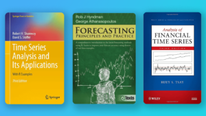
1. “Time Series Analysis and Its Applications: With R Examples” by Robert H. Shumway and David S. Stoffer: This book presents a balanced and comprehensive approach to time series analysis, with R examples. It’s ideal for anyone interested in exploring statistical methods for time series comprehensively.
2. “Forecasting: principles and Practice” by Rob J Hyndman and George Athanasopoulos: This is an excellent resource for statistical forecasting, including time series methods. It’s available for free online, but you can also purchase a hard copy.
3. “Analysis of Financial Time Series” by Ruey S. Tsay: This book provides a broad, mature, and systematic introduction to current financial econometric models and their applications to modeling and prediction of financial time series data.

Online Courses:

1. “Time Series Analysis in Python” on DataCamp: This course will guide you through everything you need to know to use Python for forecasting time series data to predict new future data points.
2. “Practical Time Series Analysis” on Coursera: Offered by the State University of New York, this course provides a practical guide to Time Series Analysis using real-world datasets.

Websites:

1. Cross Validated (Stack Exchange): This is a question-and-answer site for people interested in statistics, machine learning, data analysis, data mining, and data visualization, including plenty of content on Time Series.
2. Towards Data Science: An online platform that shares concepts on data science, AI, machine learning, and more. You can find numerous articles on Time Series Analysis from various authors.
3. The Comprehensive R Archive Network (CRAN): A collection of sites which carry identical material, consisting of the R distribution(s), the contributed extensions, documentation for R, and binaries.

Remember, the most effective way to learn is by doing. So, along with reading and taking courses, try to work on practical projects or Kaggle competitions involving Time Series Analysis. Happy learning!

Time Series Analysis FAQ:

1. Are there any assumptions made when conducting a time series analysis?

Yes, there are several assumptions made when conducting a time series analysis. Firstly, it’s assumed that the data is stationary, meaning its properties do not depend on the time at which the series is observed. Secondly, the data is assumed to be linear and normally distributed. Lastly, it’s assumed that the past is a good predictor of the future.

2. What is the difference between cross-sectional data and time series data?

Time series data is a set of observations collected sequentially over time, for instance, daily stock prices or monthly sales data. Cross-sectional data, on the other hand, is data collected on several subjects at the same point in time, such as a survey of employees’ satisfaction in a company.

3. How do I choose the appropriate forecasting model for my time series data?

Choosing the appropriate forecasting model for your time series data depends on the characteristics of your data. You would consider factors such as seasonality, trend, autocorrelation, and volatility. The model that best accounts for these features and minimizes forecast errors is usually considered the most appropriate.

4. How do I handle missing data in time series analysis?

Handling missing data in time series analysis can be challenging. Common approaches include interpolation, where a value is estimated based on neighboring data points, or imputation, where the missing values are replaced with a statistic like the mean or median. However, the best approach depends on the specifics of your data and the reasons for the missing values.

5. How does the Box-Jenkins model differ from other models in its approach to time series analysis?

The Box-Jenkins model, or ARIMA, differs from other models as it explicitly models the data as a combination of autoregressive, integrated, and moving average processes. It relies on the data being stationary and uses a systematic methodology developed by Box and Jenkins for model identification, parameter estimation, and model checking.

6. What is the main difference between ARIMA and SARIMA?

ARIMA and SARIMA models are similar, but SARIMA incorporates an additional component of seasonality. ARIMA models data with a trend, while SARIMA models data with both a trend and a seasonal component.

7. Can time series analysis techniques be applied to non-time related sequential data, like customer purchase sequences?

Yes, time series analysis techniques can be applied to non-time related sequential data. It’s often referred to as sequence analysis. Techniques like Markov Chains or sequence mining algorithms are commonly used for such data.

8. What’s the best way to validate the accuracy of my time series forecasting model?

The accuracy of a time series forecasting model is commonly validated by comparing the predicted values to the actual values using a hold-out sample. Accuracy measures like the Mean Absolute Error (MAE), Mean Squared Error (MSE), or the Mean Absolute Percentage Error (MAPE) are typically used.

9. What are the 4 components of time series?

The four main components of time series are: Trend (the overall direction of the series over time), Seasonality (the repeating short-term cycle in the series), Cycles (the long-term oscillations or patterns), and Irregularity (the random variation that can’t be attributed to the other components).

10. Why is it called a time series?

It’s called a time series because the data points are collected at regular or irregular intervals over time. The series captures the temporal order of observations, which makes it unique compared to other forms of data.

What you should know:

1. Our Mission is to Help you to Become a Professional Data Analyst.
2. This Website is a Home for Data Analysts. Get our latest in-depth Data Analysis and Artificial Intelligence Lessons and Updates in your Inbox.